Digital Earth Africa GeoMAD • vrtility

Sometimes, amazing people do all the work for you! Digital Earth Africa has a lot of amazing data available but the datasets that are (in my opinion) particularly special and, in large part, motivated the creation of vrtility (so that we can get some of the Open Data Cube functionality in R) are the GeoMAD datasets. These are (sub)annual geometric median composites of Landsat and Sentinel-2 archives for Africa. You can access these data in all manner of ways, but here is how you can do it with vrtility.

Some nice advantages of using vrtility here is - parallel asynchronous downloads and convenient organisation of the multiple bands into a single raster file.

This is also a classic use case for the VRT format, combining multiple tiles into a single file 😀.

Getting started

So let’s get into it. First load vrtility, set the number of mirai daemons you want to use (R processes that will download the data in parallel) and set some important environment variables that will allow you to access the Digital Earth Africa data from the S3 bucket. Whilst, we can provide these config options in various vrt_x commands, setting them here means you don’t have to repeat yourself.

library(vrtility)

mirai::daemons(5)
#> [1] 5


# Doing this once saves you having to add it to every vrt_x command.
Sys.setenv(
  AWS_NO_SIGN_REQUEST = "YES",
  AWS_S3_ENDPOINT = "s3.af-south-1.amazonaws.com"
)

Locating the data

To locate the data, we need to define a bounding box. First we need this bbox in lat-long coordinates for querying the STAC API, but we can project these bounds later. For convenience, we’ll use this handy function to create a bounding box from a WKT point and extend it by a certain amount in the x and y directions. This location is in North of Madagascar.

bbox <- gdalraster::bbox_from_wkt(
  wkt = "POINT (46.33 -15.9)",
  extend_x = 0.22,
  extend_y = 0.2
)

Querying the data

We can now query the STAC API for the Landsat 8 and 9 annual composites for 2024. The stac_query() function will return a doc_items object which we can use to build our VRT objects. This can be optionally filtered, as shown below, if you don’t need all of the assets (bands).

l8l9_query <- stac_query(
  bbox = bbox,
  stac_source = "https://explorer.digitalearth.africa/stac/",
  collection = "gm_ls8_ls9_annual",
  start_date = "2024-01-01",
  end_date = "2024-12-31"
)

# This step is optional - do this if you only want a subset of the assets (bands)
l8l9_query <- rstac::assets_select(
  l8l9_query,
  asset_names = c("SR_B2", "SR_B3", "SR_B4", "SR_B5")
)
print(l8l9_query)
#> ###Items
#> - matched feature(s): 2
#> - features (2 item(s) / 0 not fetched):
#>   - 6d21f993-74bc-52d3-bafa-96164e7bce86
#>   - cb7d0c9d-bc36-538b-a67d-930999cbf3c9
#> - assets: SR_B2, SR_B3, SR_B4, SR_B5
#> - item's fields: 
#> assets, bbox, collection, geometry, id, links, properties, stac_extensions, stac_version, type

Collecting the data

So now we can use the core vrtiltiy functions to collect, reproject and align (warp) the data before using vrt_compute() to create a single raster file from the VRT.

l8l9_vrt <- vrt_collect(
  l8l9_query
)

print(l8l9_vrt)
#> → <VRT Collection>
#> 
#>  VRT SRS: 
#> PROJCS["WGS 84 / NSIDC EASE-Grid 2.0 Global",GEOGCS["WGS 84",DATUM["WGS_1984",SPHEROID["WGS 84",6378137,298.257223563,AUTHORITY["EPSG","7030"]],AUTHORITY["EPSG","6326"]],PRIMEM["Greenwich",0,AUTHORITY["EPSG","8901"]],UNIT["degree",0.0174532925199433,AUTHORITY["EPSG","9122"]],AUTHORITY["EPSG","4326"]],PROJECTION["Cylindrical_Equal_Area"],PARAMETER["standard_parallel_1",30],PARAMETER["central_meridian",0],PARAMETER["false_easting",0],PARAMETER["false_northing",0],UNIT["metre",1,AUTHORITY["EPSG","9001"]],AXIS["Easting",EAST],AXIS["Northing",NORTH],AUTHORITY["EPSG","6933"]]
#> Bounding Box: 4416000 -2112000 4512000 -1920000
#> Pixel res: 30, 30
#> Start Date: 2024-01-01 UTC
#> End Date: 2024-01-01 UTC
#> Number of Items: 2
#> Assets: SR_B2, SR_B3, SR_B4, SR_B5


# if you just want to look at one of the tiles...
# plot(l8l9_vrt[[1]][[2]], c(3, 2, 1))

bbox_proj <- bbox_to_projected(bbox, l8l9_vrt$srs)

l8l9_vrt_warped <- vrt_warp(
  l8l9_vrt,
  t_srs = attr(bbox_proj, "wkt"),
  te = bbox_proj,
  tr = c(30, 30)
) |>
  vrt_stack()


l8l9file <- vrt_compute(
  l8l9_vrt_warped,
  outfile = fs::file_temp(ext = "tif"),
  engine = "gdalraster"
)

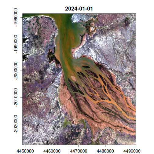
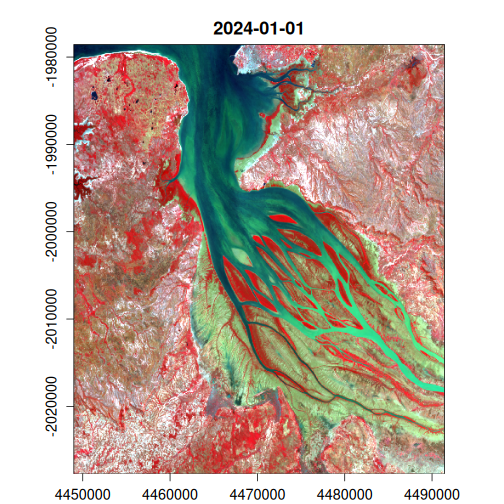
Plotting the data

Let’s have a look at the data in both true colour and false colour.

withr::with_par(list(mar = c(0, 0, 0, 0)), {
  plot_raster_src(
    l8l9file,
    bands = c(3, 2, 1),
    axes = FALSE
  )

  plot_raster_src(
    l8l9file,
    bands = c(4, 3, 2),
    axes = FALSE
  )
})