GEDI Level 1B Waveforms • chewie

This vignette demonstrates how to use the chewie package to download and extract GEDI Level 1B waveforms.

First let’s load the chewie package and the ggplot2 package for plotting.

library(chewie)
library(ggplot2)
library(sf)
library(dplyr)

First, we define an area of interest. In this case, we will use prairie creek national park as our area of interest. The chewie package provides a number of example spatial vector data sets that can be used for this purpose. Here we use the prairie-creek.geojson data set, which is a simple polygon defining the park boundary. You can alternatively use the st_read() function to read in your own spatial vector data.

pcreek <- system.file(
  "geojson", "prairie-creek.geojson",
  package = "chewie"
) |>
  sf::read_sf()

Now we can search for GEDI Level 1B products that intersect with our area of interest. We will search for products that were collected between January 1st and January 31st, 2023.

g1b_search <- find_gedi(pcreek,
  gedi_product = "1B",
  date_start = "2023-01-01",
  date_end = "2023-01-31"
)
#> ✔ Using cached GEDI find result
print(g1b_search)
#> 
#> ── chewie.find ───────────────────────────────────────────────────────────────────────────────────────────────────────────────────
#> • GEDI-1B
#>                     id          time_start            time_end                                                   url cached
#>                 <char>              <POSc>              <POSc>                                                <char> <lgcl>
#> 1: G2755093540-LPCLOUD 2023-01-25 05:14:31 2023-01-25 06:47:21 https://data.lpdaac.earthdatacloud.nasa.gov/lp-pro...   TRUE
#> 1 variable(s) not shown: [geometry <sfc_POLYGON>]
#> 
#> ──────────────────────────────────────────────────────────────────────────────────────────────────────────────────────────────────

You’ll see that only one granule was found. The returned gedi.find object contains information about the search, including whether or not the files are cached locally.

Note: this vignette uses a cached granule which has been subset to include only 3 beams to minimise the size of the package. The full granule contains 8 beams.

Now we can download the GEDI Level 1B products. However, note that the grab_gedi() function will not download the products if they are already cached locally. It first checks the cache and grabs the relevant files if they exist. If they do not exist, they’ll be downloaded from the LPCLOUD bucket. {chewie} will, by default only download specific data columns. There are many variables contained in the raw hdf5 files.

gedi_1b_arrow <- grab_gedi(g1b_search)
#> ✔ All data found in cache

The grab_gedi() function returns a arrow_dplyr_query object. If the user wishes to carry out further filtering (for example using quality flags), this should be done at this stage to avoid loading unnecessary data into memory.

In order to access the data we must first collect the data into a data frame. This could be done using dplyr::collect. However, the collect_gedi() function is a wrapper around dplyr::collect that also converts the data to an sf object, immediately providing a spatial context for the data.

g1b_sf <- collect_gedi(gedi_1b_arrow, g1b_search)

print(g1b_sf)
#> Simple feature collection with 349 features and 82 fields
#> Geometry type: POINT
#> Dimension:     XY
#> Bounding box:  xmin: -124.0638 ymin: 41.39252 xmax: -123.9959 ymax: 41.43934
#> Geodetic CRS:  WGS 84
#> # A tibble: 349 × 83
#>    all_samples_sum  beam channel delta_time date_time           master_frac
#>  *           <int> <int>   <int>      <dbl> <dttm>                    <dbl>
#>  1        15740038     2       1 159862145. 2023-01-25 06:09:04       0.844
#>  2        15757882     2       1 159862145. 2023-01-25 06:09:04       0.852
#>  3        15758137     2       1 159862145. 2023-01-25 06:09:04       0.860
#>  4        15771162     2       1 159862145. 2023-01-25 06:09:04       0.868
#>  5        15761837     2       1 159862145. 2023-01-25 06:09:04       0.877
#>  6        15744387     2       1 159862145. 2023-01-25 06:09:04       0.885
#>  7        15746553     2       1 159862145. 2023-01-25 06:09:04       0.893
#>  8        15766075     2       1 159862145. 2023-01-25 06:09:04       0.901
#>  9        15750489     2       1 159862145. 2023-01-25 06:09:04       0.910
#> 10        15737307     2       1 159862145. 2023-01-25 06:09:04       0.918
#> # ℹ 339 more rows
#> # ℹ 77 more variables: master_int <int>, noise_mean_corrected <dbl>,
#> #   noise_stddev_corrected <dbl>, nsemean_even <dbl>, nsemean_odd <dbl>,
#> #   rx_energy <dbl>, rx_offset <int>, rx_open <int>, rx_sample_count <int>,
#> #   rx_sample_start_index <int>, selection_stretchers_x <int>,
#> #   selection_stretchers_y <int>, shot_number <chr>, stale_return_flag <int>,
#> #   th_left_used <int>, tx_egamplitude <dbl>, tx_egamplitude_error <dbl>, …

ggplot() +
  geom_sf(data = attributes(g1b_search)$aoi, fill = "#1bbe8086") +
  geom_sf(data = g1b_sf, aes(colour = elevation_lastbin)) +
  guides(colour = "none") +
  scale_color_viridis_c(option = "A") +
  theme_light()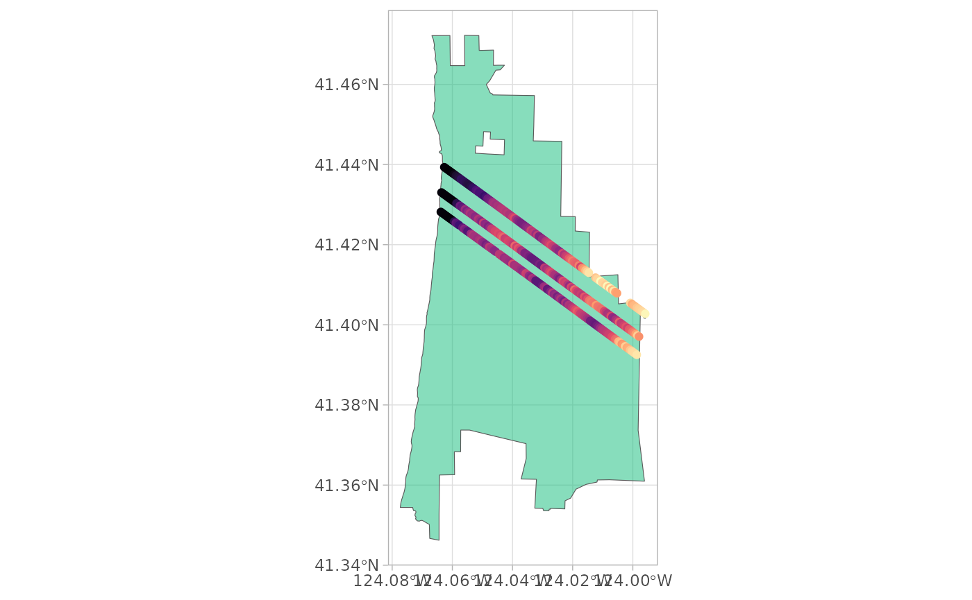

So, here’s the cool bit about the way the Level-1B data are extracted. We can access the full waveform for every shot in the data set by using the extract_waveforms() function. This generates a long-form data frame with waveform amplitude, relative elevation, and shot number for each shot. This enables the combined analysis and comparison of many waveforms across space (and time when we have multiple granules).

For example, here we take 8 of the waveforms…

g1b_wvf <- extract_waveforms(g1b_sf[100:108, ])

print(g1b_wvf)
#> # A tibble: 10,204 × 4
#>    shot_number        date_time           rxelevation rxwaveform
#>    <chr>              <dttm>                    <dbl>      <dbl>
#>  1 233300200300278449 2023-01-25 06:09:05        328.       239.
#>  2 233300200300278449 2023-01-25 06:09:05        328.       239.
#>  3 233300200300278449 2023-01-25 06:09:05        328.       238.
#>  4 233300200300278449 2023-01-25 06:09:05        328.       238.
#>  5 233300200300278449 2023-01-25 06:09:05        328.       239.
#>  6 233300200300278449 2023-01-25 06:09:05        328.       239.
#>  7 233300200300278449 2023-01-25 06:09:05        328.       240.
#>  8 233300200300278449 2023-01-25 06:09:05        327.       241.
#>  9 233300200300278449 2023-01-25 06:09:05        327.       241.
#> 10 233300200300278449 2023-01-25 06:09:05        327.       241.
#> # ℹ 10,194 more rows

And plot them using ggplot2…

wvf_ggplot <- function(x, wf, z, .ylab = "Elevation (m)") {
  wf <- sym(wf)
  z <- sym(z)
  ggplot(x, aes(x = !!z, y = !!wf)) +
    geom_ribbon(aes(ymin = min(!!wf), ymax = !!wf),
      alpha = 0.6, fill = "#69d66975", colour = "grey30", lwd = 0.2
    ) +
    theme_light() +
    coord_flip() +
    labs(x = .ylab, y = "Waveform Amplitude")
}

wvf_ggplot(g1b_wvf, "rxwaveform", "rxelevation") +
  facet_wrap(~shot_number, ncol = 5, scales = "free")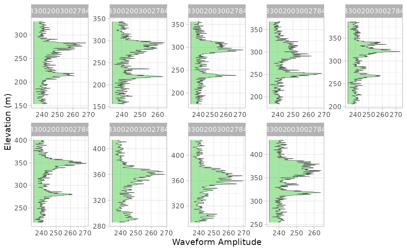

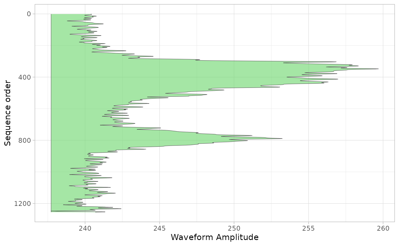
We can also calculate the mean waveform for these shots and plot it. Note that this may not be particualtly helpful for all contexts, but it provides an indication of the power of having access to all waveforms in a single dataset.

g1b_wvf |>
  group_by(shot_number) |>
  arrange(rxelevation) |>
  mutate(id = dplyr::n():1) |>
  ungroup() |>
  group_by(id) |>
  summarise(
    mean_wvf = mean(rxwaveform),
    mean_elev = mean(rxelevation)
  ) |>
  wvf_ggplot("mean_wvf", "id", .ylab = "Sequence order") +
  scale_x_reverse()