How can I...?

This vignette aims to provide a “cookbook” walking through common use cases and code patterns for rsi. If you’ve got a problem that it seems like rsi should be able to solve, hopefully this document can help – otherwise, open an issue and we’ll see if we can get you started! And if you’ve got a use case that took you a second to figure out, please feel free to open a PR to add it as an example to this document.

With that introduction out of the way, we’ll go ahead and load rsi:

library(rsi)

And start answering: How can I…

Get one composite per year, month, or other interval?

If you’re looking to get separate files for several intervals, you’ll need to call get_stac_data() separately for each of those intervals. The easiest way to do this is through something like vapply() or a for-loop. Iterate along your intervals of interest, construct your start_date and end_date inside of each iteration, and call get_stac_data() using those dates as arguments:

aoi <- sf::st_point(c(-74.912131, 44.080410))
aoi <- sf::st_set_crs(sf::st_sfc(aoi), 4326)
aoi <- sf::st_buffer(sf::st_transform(aoi, 5070), 1000)

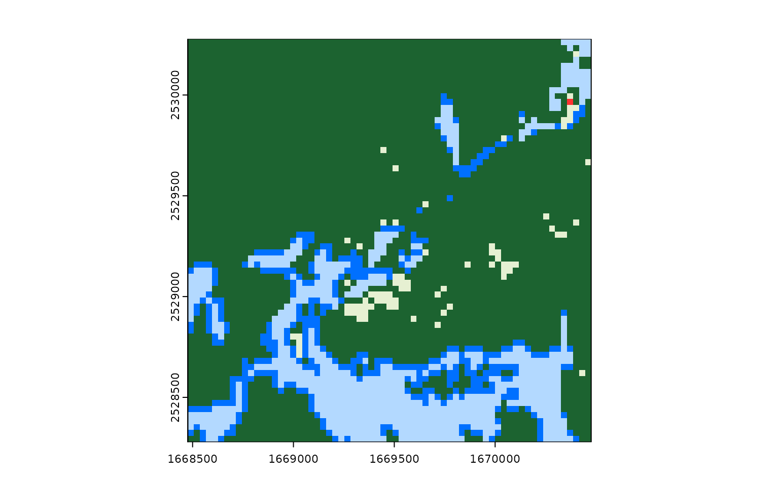
downloaded_years <- vapply(
  2018:2020,
  function(year) {
    get_stac_data(
      aoi = aoi,
      start_date = glue::glue("{year}-01-01"),
      end_date = glue::glue("{year}-12-31"),
      asset_names = "lcpri",
      stac_source = "https://planetarycomputer.microsoft.com/api/stac/v1",
      collection = "usgs-lcmap-conus-v13",
      output_filename = file.path(tempdir(), glue::glue("{year}.tif"))
    )
  },
  character(1)
)

downloaded_years
#> [1] "/tmp/RtmpwHJdDK/2018.tif" "/tmp/RtmpwHJdDK/2019.tif"
#> [3] "/tmp/RtmpwHJdDK/2020.tif"

This ensures that get_stac_data() is run using the same arguments each time, so your outputs should be standardized across each interval!

invisible(lapply(lapply(downloaded_years, terra::rast), terra::plot))

Get each distinct item that matches a query, without compositing?

If we want to download the individual STAC items that are returned by our query, we can set the composite_function argument to NULL. This will return one file per STAC item, with the datetime element of the item appended to the filename if it exists (and a sequential identifier if it doesn’t):

aoi <- sf::st_point(c(-74.912131, 44.080410))
aoi <- sf::st_set_crs(sf::st_sfc(aoi), 4326)
aoi <- sf::st_buffer(sf::st_transform(aoi, 5070), 1000)

our_imagery <- get_landsat_imagery(
  aoi,
  start_date = "2023-06-01",
  end_date = "2023-07-01",
  output_filename = tempfile(fileext = ".tif"),
  composite_function = NULL
)

our_imagery
#> [1] "/tmp/RtmpwHJdDK/file25ec54c1938a_2023-06-28T154415.862937Z.tif"
#> [2] "/tmp/RtmpwHJdDK/file25ec54c1938a_2023-06-20T154419.579981Z.tif"
#> [3] "/tmp/RtmpwHJdDK/file25ec54c1938a_2023-06-12T154413.224112Z.tif"
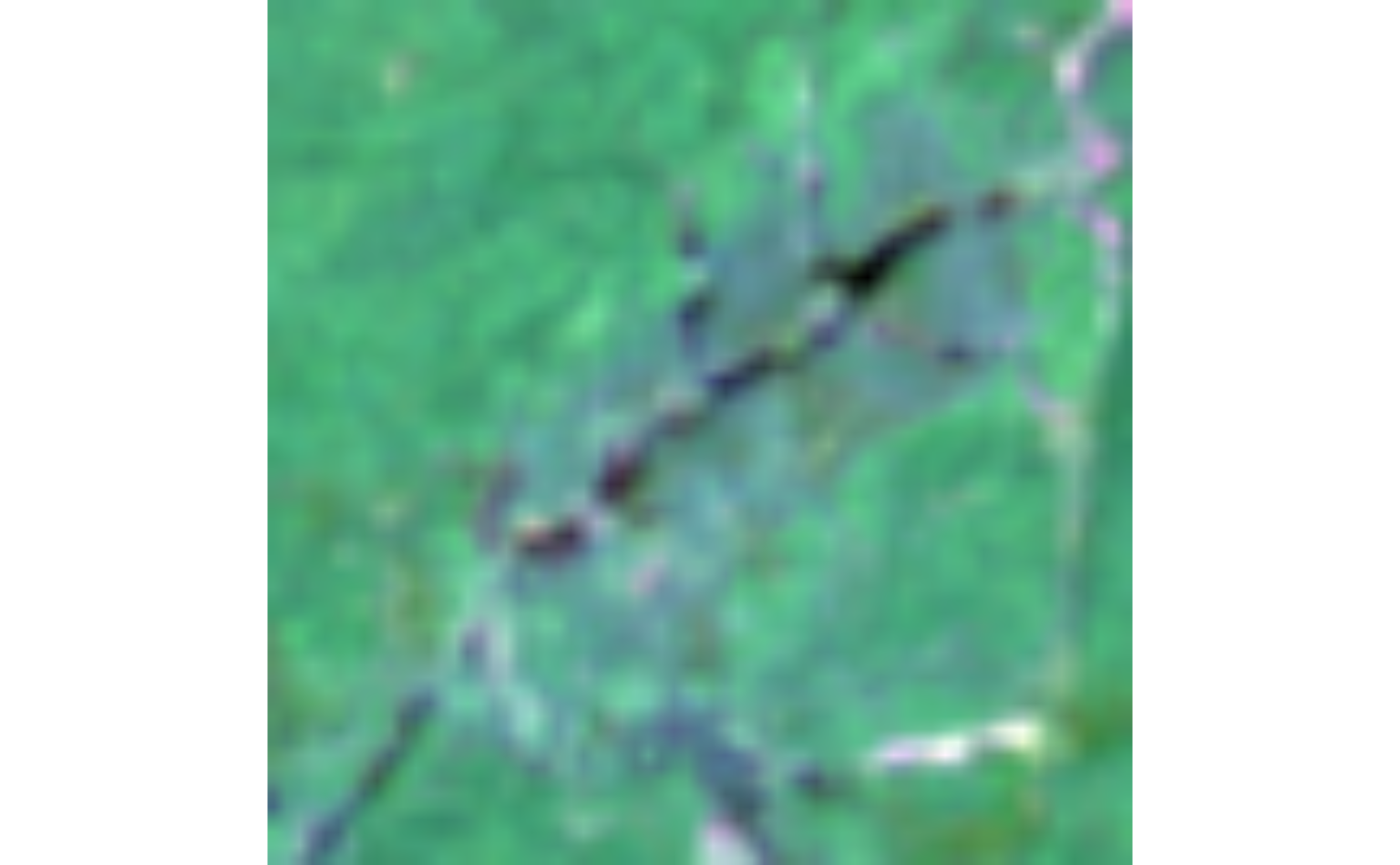
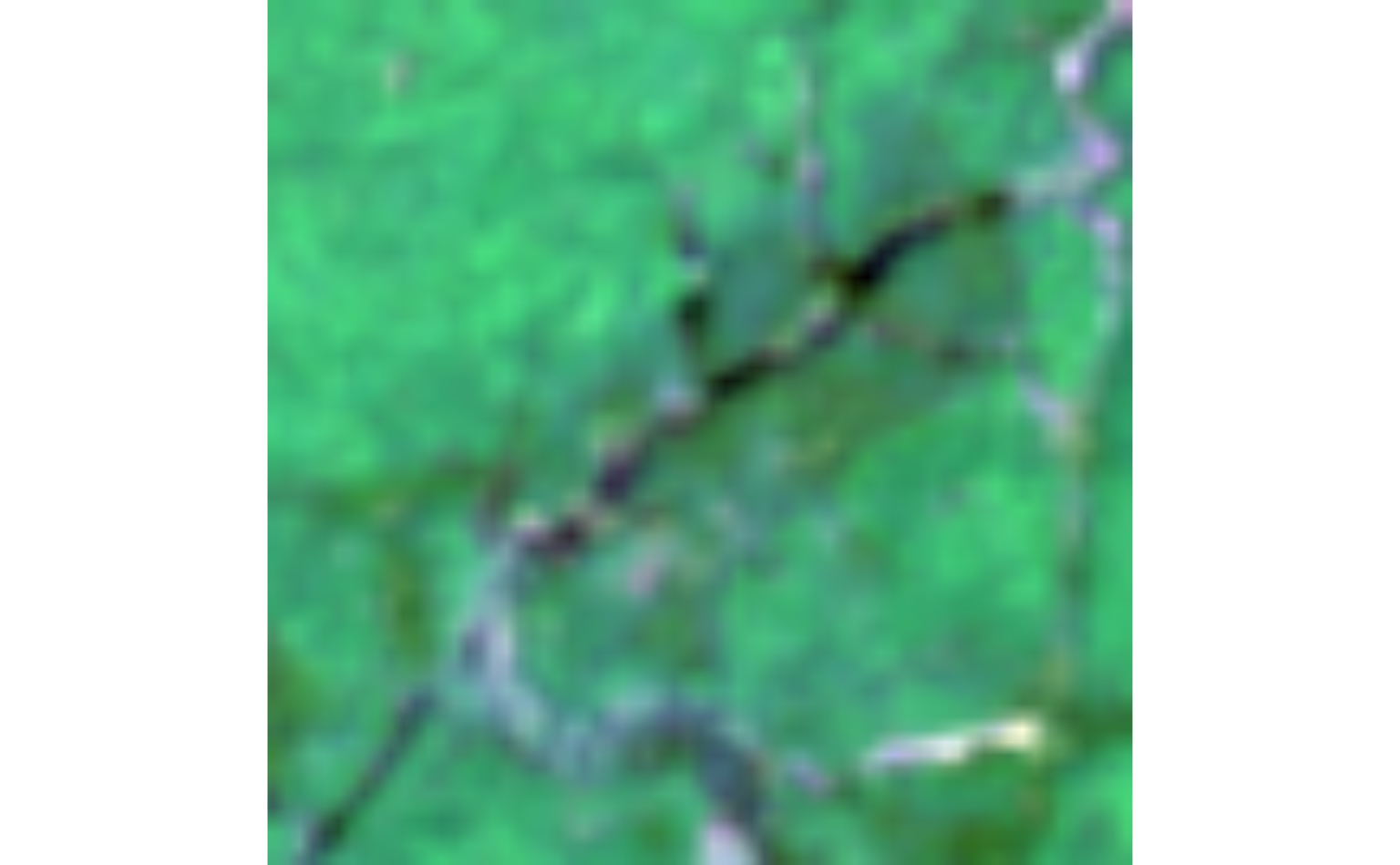
#> [4] "/tmp/RtmpwHJdDK/file25ec54c1938a_2023-06-04T154412.531019Z.tif"

Each of these files will then contain the assets corresponding to that individual STAC item:

terra::rast(our_imagery[[2]], lyrs = c("R", "G", "B")) |>
  terra::stretch() |>
  terra::plotRGB()

terra::rast(our_imagery[[4]], lyrs = c("R", "G", "B")) |>
  terra::stretch() |>
  terra::plotRGB()

Filter the imagery I download by cloud cover (or other metadata)?

If you want to refine the outputs from your STAC query, the best approach is to write a custom query function using CQL2. CQL2 is a complicated topic, which is covered in a bit more detail both in the Downloading Data vignette as well as in the STAC website’s tutorials, but at its core is a query language that lets us filter our results down using a spatiotemporal area of interest as well as other item-level metadata.

This requires knowing what metadata your STAC API provides for the items you’re querying! Luckily, a good number of these fields are standardized via the STAC standard and various STAC extensions. For instance, items implementing the electro-optical extension will have an eo:cloud_cover field which we could use to filter the results of our query.

Writing a query function to filter using this field might look like this:

aoi <- sf::st_point(c(-74.912131, 44.080410))
aoi <- sf::st_set_crs(sf::st_sfc(aoi), 4326)
aoi <- sf::st_buffer(sf::st_transform(aoi, 5070), 1000)

custom_query_function <- function(bbox, 
                                  stac_source, 
                                  collection, 
                                  start_date, 
                                  end_date, 
                                  limit, 
                                  ...) {
  geometry <- rstac::cql2_bbox_as_geojson(bbox) 
  datetime <- rstac::cql2_interval(start_date, end_date)
  
  request <- rstac::ext_filter(
    rstac::stac(stac_source),
    collection == {{collection}} &&
      t_intersects(datetime, {{datetime}}) &&
      s_intersects(geometry, {{geometry}}) && 
      `eo:cloud_cover` < 50
  )
  rstac::items_fetch(rstac::post_request(request))
}

And we can use this to filter down how much data we’ll download! For instance, we could download Landsat imagery for our area of interest without using our new query function and setting composite_function to NULL, so that we’ll get one file per Landsat image:

unfiltered_landsat_images <- get_landsat_imagery(
  aoi,
  start_date = "2023-06-01",
  end_date = "2023-09-01",
  # Only downloading one asset, because we aren't using this data for anything
  asset_names = landsat_band_mapping$planetary_computer_v1["red"],
  mask_function = NULL,
  mask_band = NULL,
  output_filename = tempfile(fileext = ".tif"),
  composite_function = NULL
)
length(unfiltered_landsat_images)
#> [1] 12

And we could compare that to a query using our custom query function, to see how many images are filtered out by our CQL2 query:

filtered_landsat_images <- get_landsat_imagery(
  aoi,
  start_date = "2023-06-01",
  end_date = "2023-09-01",
  query_function = custom_query_function,
  asset_names = landsat_band_mapping$planetary_computer_v1["red"],
  mask_function = NULL,
  mask_band = NULL,
  output_filename = tempfile(fileext = ".tif"),
  composite_function = NULL
)
length(filtered_landsat_images)
#> [1] 7

We only wind up downloading about half the number of images!

Calculate all possible indices using a certain data set?

Say you’ve got some imagery:

aoi <- sf::st_point(c(-74.912131, 44.080410))
aoi <- sf::st_set_crs(sf::st_sfc(aoi), 4326)
aoi <- sf::st_buffer(sf::st_transform(aoi, 5070), 1000)

our_imagery <- get_landsat_imagery(
  aoi,
  start_date = "2023-06-01",
  end_date = "2023-07-01",
  output_filename = tempfile(fileext = ".tif")
)

You want to calculate some indices from this imagery. Specifically, you want to calculate all the indices you can from this imagery – you’re doing some sort of machine learning/data mining work, and you want to throw as many indices in the mix as possible.

To do that using calculate_indices(), you’re going to need to only provide formulas for the indices that can be calculated from your particular data source. We might look at the columns available for filtering from spectral_indices():

spectral_indices() |> 
  head(1)
#> # A tibble: 1 × 9
#>   application_domain bands     contributor    date_of_addition formula long_name
#>   <chr>              <list>    <chr>          <chr>            <chr>   <chr>    
#> 1 vegetation         <chr [2]> https://githu… 2021-11-17       (N - 0… Aerosol …
#> # ℹ 3 more variables: platforms <list>, reference <chr>, short_name <chr>

It might seem like we’d want to use the platforms column here: we just downloaded a bunch of data from the Landsat-OLI platform, so we probably want to calculate indices that correspond to this platform. Unfortunately, if we use filter_platforms() to do this filtering, we’ll get an error inside of calculate_indices():

try(
  calculate_indices(
    our_imagery,
    filter_platforms(platforms = "Landsat-OLI"),
    output_filename = tempfile(fileext = ".tif")
  )
)
#> Error in eval(calc) : object 'gamma' not found

The issue is that a number of the indices in the Awesome Spectral Indices project have formulas that require additional data. You can see a list of them in the ASI documentation described as “additional index parameters”, and they range from wavelength values to exponentiation factors to weighting parameters and so on.

If you care about using a specific index, then it’s your job to figure out what extra parameters that index requires and how you’ll provide them. The spectral_indices() table also includes a DOI to the authoritative reference (as listed in the ASI project) which can hopefully help with this.

However, if you’re looking to automatically calculate just the indices that don’t require external parameters, you can do that as well. Rather than use filter_platforms(), we’ll use filter_bands() to retrieve all the spectral indices that can be calculated using the bands available in our raster.

Assuming you used one of the wrapper functions in rsi, like get_landsat_data() or get_sentinel2_data(), your raster bands should automatically be named to match the band names used in the ASI project. That means we can pass the names of your raster directly to filter_bands():

filter_bands(bands = names(terra::rast(our_imagery))) |> 
  head(1)
#> # A tibble: 1 × 9
#>   application_domain bands     contributor    date_of_addition formula long_name
#>   <chr>              <list>    <chr>          <chr>            <chr>   <chr>    
#> 1 vegetation         <chr [2]> https://githu… 2021-11-17       (N - 0… Aerosol …
#> # ℹ 3 more variables: platforms <list>, reference <chr>, short_name <chr>

And we can pass the outputs of that function to calculate_indices() to only calculate this subset of indices:

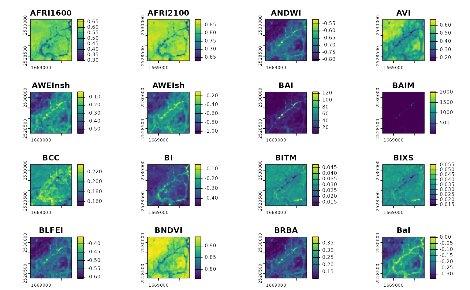
calculate_indices(
    our_imagery,
    filter_bands(bands = names(terra::rast(our_imagery))),
    output_filename = tempfile(fileext = ".tif")
  ) |> 
  terra::rast() |> 
  terra::plot()
#> Warning in x@ptr$writeStop(): GDAL Message 1:
#> /tmp/RtmpwHJdDK/file25ec7b3f9aa.tif: Metadata exceeding 32000 bytes cannot be
#> written into GeoTIFF. Transferred to PAM instead.