Data Structures and Terminology • vrtility

library(vrtility)
#> ✔ Using GDAL version 3.8.4
#> ℹ GDAL_CACHEMAX set to 1.562 GiB; to change this use
#>   vrtility::set_gdal_cache_max()

Overview

The vrtility package is built around three core data structures that represent virtual rasters at different levels of organization: vrt_block, vrt_collection, and vrt_stack. Understanding these structures is key to working effectively with the package’s VRT-based pipelines. Figure 1 provides a visual overview of these data structures and their relationships. which are discussed in detail below.

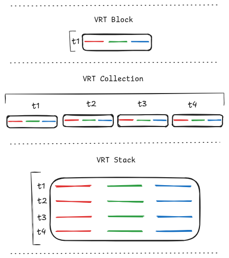
Figure 1: Core data structures in vrtility: vrt_block, vrt_collection, and vrt_stack. Red, green, and blue lines represent raster bands; black boxes represent VRT files; t* labels indicate discrete epochs (time steps).

There is considerable jargon in the GIS world regarding multidimensional raster data. The term “data cube” is commonly used for spatiotemporal rasters, but we feel this metaphor breaks down for multiband/multi-spectral data. In reality, we have interconnected “cubes” linked by a space-time index. We prefer “stack” over “cube” when referring to the temporal dimension of our data, aligning with GDAL terminology and establishing a clearer mental model.

However, “stacking” sometimes refers to adding bands to a multiband raster. For clarity: in vrtility, “stack” always refers to aligning bands representing the same phenomenon across multiple time steps into a single virtual raster.

Core Data Structures

vrt_block: The Basic Building Block 😉

A vrt_block represents a single virtual raster (VRT) with one or more bands. It is the fundamental unit in vrtility’s pipeline system.

Key characteristics:

Contains a single VRT XML definition
Has a single spatial reference system (SRS)
Contains one or more raster bands (e.g., B02, B03, B04)
Can be created from one or more data sources.
May include metadata like timestamps and no-data values
Stores optional mask and pixel functions

# Load example Sentinel-2 data
s2files <- fs::dir_ls(system.file("s2-data", package = "vrtility"))

# Create a vrt_collection and extract the first block
ex_collect <- vrt_collect(s2files, datetimes = c(
  "2020-01-01T10:15:30Z", # dates made up for example
  "2020-02-01T10:15:30Z",
  "2020-03-01T10:15:30Z",
  "2020-04-01T10:15:30Z",
  "2020-05-01T10:15:30Z"
))
single_block <- ex_collect[[1]][[1]]

# Print the block to see its structure
print(single_block)
#> → <VRT Block>
#> VRT XML: [hidden]
#>   run print(x, xml = TRUE) to view
#> 
#>  VRT SRS: 
#> PROJCS["OSGB36 / British National Grid",GEOGCS["OSGB36",DATUM["Ordnance_Survey_of_Great_Britain_1936",SPHEROID["Airy 1830",6377563.396,299.3249646,AUTHORITY["EPSG","7001"]],AUTHORITY["EPSG","6277"]],PRIMEM["Greenwich",0,AUTHORITY["EPSG","8901"]],UNIT["degree",0.0174532925199433,AUTHORITY["EPSG","9122"]],AUTHORITY["EPSG","4277"]],PROJECTION["Transverse_Mercator"],PARAMETER["latitude_of_origin",49],PARAMETER["central_meridian",-2],PARAMETER["scale_factor",0.9996012717],PARAMETER["false_easting",400000],PARAMETER["false_northing",-100000],UNIT["metre",1,AUTHORITY["EPSG","9001"]],AXIS["Easting",EAST],AXIS["Northing",NORTH],AUTHORITY["EPSG","27700"]]
#> 
#> 
#> Bounding Box: 289813.58 88876.43 297031.04 95714.02
#> Pixel res: 19.9929669011164, 19.9929669011164
#> Assets: B02, B03, B04, B08, SCL
#> No Data Value(s): 0, 0, 0, 0, 0
#> Date Time: 2020-01-01 10:15:30 UTC

A vrt_block contains:

vrt: The XML representation of the VRT
vrt_src: Path to the VRT file
srs: Spatial reference system
bbox: Bounding box (extent)
res: Pixel resolution
assets: Band names (e.g., “B02”, “B03”, “B04”)
date_time: Timestamp(s)
no_data_val: NoData value(s) for each band
pixfun: Optional pixel function code
maskfun: Optional mask function code
warped: Whether the VRT has been spatially aligned
is_remote: Whether the data source is remote (e.g., S3)

vrt_collection: Temporal Series of Blocks

A vrt_collection is a list of vrt_block objects, typically representing a time series of observations over the same geographic area.

Key characteristics:

Contains multiple vrt_block objects (e.g., t1, t2, t3, t4)
Each block typically has the same set of bands (e.g., B02, B03, B04)
Blocks may have different timestamps
Blocks may have different spatial references and extents until warped
Component blocks can be warped to a common grid using vrt_warp()
Inherits from vrt_block, so supports the same operations

# Print collection summary
print(ex_collect)
#> → <VRT Collection>
#> 
#>  VRT SRS: 
#> PROJCS["OSGB36 / British National Grid",GEOGCS["OSGB36",DATUM["Ordnance_Survey_of_Great_Britain_1936",SPHEROID["Airy 1830",6377563.396,299.3249646,AUTHORITY["EPSG","7001"]],AUTHORITY["EPSG","6277"]],PRIMEM["Greenwich",0,AUTHORITY["EPSG","8901"]],UNIT["degree",0.0174532925199433,AUTHORITY["EPSG","9122"]],AUTHORITY["EPSG","4277"]],PROJECTION["Transverse_Mercator"],PARAMETER["latitude_of_origin",49],PARAMETER["central_meridian",-2],PARAMETER["scale_factor",0.9996012717],PARAMETER["false_easting",400000],PARAMETER["false_northing",-100000],UNIT["metre",1,AUTHORITY["EPSG","9001"]],AXIS["Easting",EAST],AXIS["Northing",NORTH],AUTHORITY["EPSG","27700"]]
#> 
#>  PROJCS["WGS 84 / UTM zone 30N",GEOGCS["WGS 84",DATUM["WGS_1984",SPHEROID["WGS 84",6378137,298.257223563,AUTHORITY["EPSG","7030"]],AUTHORITY["EPSG","6326"]],PRIMEM["Greenwich",0,AUTHORITY["EPSG","8901"]],UNIT["degree",0.0174532925199433,AUTHORITY["EPSG","9122"]],AUTHORITY["EPSG","4326"]],PROJECTION["Transverse_Mercator"],PARAMETER["latitude_of_origin",0],PARAMETER["central_meridian",-3],PARAMETER["scale_factor",0.9996],PARAMETER["false_easting",500000],PARAMETER["false_northing",0],UNIT["metre",1,AUTHORITY["EPSG","9001"]],AXIS["Easting",EAST],AXIS["Northing",NORTH],AUTHORITY["EPSG","32630"]]
#> 
#>  PROJCS["unknown",GEOGCS["unknown",DATUM["Unknown based on WGS 84 ellipsoid",SPHEROID["WGS 84",6378137,298.257223563,AUTHORITY["EPSG","7030"]]],PRIMEM["Greenwich",0],UNIT["degree",0.0174532925199433,AUTHORITY["EPSG","9122"]]],PROJECTION["Lambert_Azimuthal_Equal_Area"],PARAMETER["latitude_of_center",50.72],PARAMETER["longitude_of_center",-3.51],PARAMETER["false_easting",0],PARAMETER["false_northing",0],UNIT["metre",1],AXIS["Easting",EAST],AXIS["Northing",NORTH]]
#> 
#> 
#> Bounding Box: NA
#> Pixel res: 19.9923198138287, 19.9923198138287
#> Start Date: 2020-01-01 10:15:30 UTC
#> End Date: 2020-05-01 10:15:30 UTC
#> Number of Items: 5
#> Assets: B02, B03, B04, B08, SCL

# A collection is a list of blocks
length(ex_collect[[1]])
#> [1] 5

# Access individual blocks
print(ex_collect[[1]][[1]]) # First time step
#> → <VRT Block>
#> VRT XML: [hidden]
#>   run print(x, xml = TRUE) to view
#> 
#>  VRT SRS: 
#> PROJCS["OSGB36 / British National Grid",GEOGCS["OSGB36",DATUM["Ordnance_Survey_of_Great_Britain_1936",SPHEROID["Airy 1830",6377563.396,299.3249646,AUTHORITY["EPSG","7001"]],AUTHORITY["EPSG","6277"]],PRIMEM["Greenwich",0,AUTHORITY["EPSG","8901"]],UNIT["degree",0.0174532925199433,AUTHORITY["EPSG","9122"]],AUTHORITY["EPSG","4277"]],PROJECTION["Transverse_Mercator"],PARAMETER["latitude_of_origin",49],PARAMETER["central_meridian",-2],PARAMETER["scale_factor",0.9996012717],PARAMETER["false_easting",400000],PARAMETER["false_northing",-100000],UNIT["metre",1,AUTHORITY["EPSG","9001"]],AXIS["Easting",EAST],AXIS["Northing",NORTH],AUTHORITY["EPSG","27700"]]
#> 
#> 
#> Bounding Box: 289813.58 88876.43 297031.04 95714.02
#> Pixel res: 19.9929669011164, 19.9929669011164
#> Assets: B02, B03, B04, B08, SCL
#> No Data Value(s): 0, 0, 0, 0, 0
#> Date Time: 2020-01-01 10:15:30 UTC
print(ex_collect[[1]][[2]]) # Second time step
#> → <VRT Block>
#> VRT XML: [hidden]
#>   run print(x, xml = TRUE) to view
#> 
#>  VRT SRS: 
#> PROJCS["WGS 84 / UTM zone 30N",GEOGCS["WGS 84",DATUM["WGS_1984",SPHEROID["WGS 84",6378137,298.257223563,AUTHORITY["EPSG","7030"]],AUTHORITY["EPSG","6326"]],PRIMEM["Greenwich",0,AUTHORITY["EPSG","8901"]],UNIT["degree",0.0174532925199433,AUTHORITY["EPSG","9122"]],AUTHORITY["EPSG","4326"]],PROJECTION["Transverse_Mercator"],PARAMETER["latitude_of_origin",0],PARAMETER["central_meridian",-3],PARAMETER["scale_factor",0.9996],PARAMETER["false_easting",500000],PARAMETER["false_northing",0],UNIT["metre",1,AUTHORITY["EPSG","9001"]],AXIS["Easting",EAST],AXIS["Northing",NORTH],AUTHORITY["EPSG","32630"]]
#> 
#> 
#> Bounding Box: 460436.9 5615438.2 467554.2 5622175.6
#> Pixel res: 19.9923198138287, 19.9923198138287
#> Assets: B02, B03, B04, B08, SCL
#> No Data Value(s): 0, 0, 0, 0, 0
#> Date Time: 2020-02-01 10:15:30 UTC

A vrt_collection extends vrt_block with:

n_items: Number of blocks in the collection
List structure where [[1]] or $vrt contains the blocks
Aggregated metadata from all blocks (e.g., combined timestamps)

Common workflow:

Note that when we print the warped collection, we see that the collections bounding box is returned rather than NA, indicating that the collection has been warped to a common grid.

# 2. Apply transformations (masking, scaling)
ex_masked <- ex_collect |>
  vrt_set_maskfun(
    mask_band = "SCL",
    mask_values = c(0, 1, 2, 3, 8, 9, 10, 11)
  )

# 3. Align to common grid
t_block <- ex_collect[[1]][[1]]
ex_warped <- vrt_warp(
  ex_masked,
  t_srs = t_block$srs,
  te = t_block$bbox,
  tr = t_block$res
)

print(ex_warped)
#> → <VRT Collection>
#> Mask Function: [hidden]
#>   run print(x, maskfun = TRUE) to view
#> 
#>  VRT SRS: 
#> PROJCS["OSGB36 / British National Grid",GEOGCS["OSGB36",DATUM["Ordnance_Survey_of_Great_Britain_1936",SPHEROID["Airy 1830",6377563.396,299.3249646,AUTHORITY["EPSG","7001"]],AUTHORITY["EPSG","6277"]],PRIMEM["Greenwich",0,AUTHORITY["EPSG","8901"]],UNIT["degree",0.0174532925199433,AUTHORITY["EPSG","9122"]],AUTHORITY["EPSG","4277"]],PROJECTION["Transverse_Mercator"],PARAMETER["latitude_of_origin",49],PARAMETER["central_meridian",-2],PARAMETER["scale_factor",0.9996012717],PARAMETER["false_easting",400000],PARAMETER["false_northing",-100000],UNIT["metre",1,AUTHORITY["EPSG","9001"]],AXIS["Easting",EAST],AXIS["Northing",NORTH],AUTHORITY["EPSG","27700"]]
#> 
#> 
#> Bounding Box: 289813.58 88876.43 297031.04 95714.02
#> Pixel res: 19.9929669011164, 19.9929669011164
#> Start Date: 2020-01-01 10:15:30 UTC
#> End Date: 2020-05-01 10:15:30 UTC
#> Number of Items: 5
#> Assets: B02, B03, B04, B08

# 4. Compute or stack for further processing

There are two functions which only support vrt_collection objects: - multiband_reduce(): Apply band reductions that require information from across the band range (e.g. geometric median or medoid). - singleband_m2m(): Apply time-series pixel functions that operate across time steps.

In these cases, the collection structure better supports data access because, these operations are carried out by R, rather than GDAL.

vrt_stack: Transposed Multi-Temporal View

A vrt_stack reorganizes a vrt_collection by stacking all time steps into a single VRT with multiple sources per original band.

Key characteristics: - Transposes the collection structure: think of a vrt collection being like a table with a wide format and the stack being the long format.

If a collection has 4 time steps and three bands, the resulting stack will have 3 bands each with 4 sources (one per time step).
Bands are grouped by original band name (all B02, then all B03, etc.)
Enables temporal operations (e.g., median, mean) across time. Note this can only be done at the band-level only, not across bands as in multiband_reduce().
Single VRT file representing the entire time series

# Stack a warped collection
ex_stack <- vrt_stack(ex_warped)

# Print stack info
print(ex_stack)
#> → VRT STACK
#> VRT XML: [hidden]
#>   run print(x, xml = TRUE) to view
#> Mask Function: [hidden]
#>   run print(x, maskfun = TRUE) to view
#> 
#>  VRT SRS: 
#> PROJCS["OSGB36 / British National Grid",GEOGCS["OSGB36",DATUM["Ordnance_Survey_of_Great_Britain_1936",SPHEROID["Airy 1830",6377563.396,299.3249646,AUTHORITY["EPSG","7001"]],AUTHORITY["EPSG","6277"]],PRIMEM["Greenwich",0,AUTHORITY["EPSG","8901"]],UNIT["degree",0.0174532925199433,AUTHORITY["EPSG","9122"]],AUTHORITY["EPSG","4277"]],PROJECTION["Transverse_Mercator"],PARAMETER["latitude_of_origin",49],PARAMETER["central_meridian",-2],PARAMETER["scale_factor",0.9996012717],PARAMETER["false_easting",400000],PARAMETER["false_northing",-100000],UNIT["metre",1,AUTHORITY["EPSG","9001"]],AXIS["Easting",EAST],AXIS["Northing",NORTH],AUTHORITY["EPSG","27700"]]
#> 
#> 
#> Bounding Box: 289813.58 88876.43 297031.04 95714.02
#> Start Date: 2020-01-01 10:15:30 UTC
#> End Date: 2020-05-01 10:15:30 UTC
#> Number of Items: 5
#> Assets: B02, B03, B04, B08

# A stack consolidates all time steps into bands
# If collection had 4 dates × 3 bands = 12 bands in stack

Structure comparison:

This table summarizes the differences between the three data structures for a typical STAC collection using Cloud Optimized GeoTIFFs for each asset.

Structure	Organization	Example (4 dates, 3 bands)
`vrt_block`	1 VRT file; N bands; N sources	[B02, B03, B04]
`vrt_collection`	M VRT files; N bands; N sources	t1: [B02, B03, B04] t2: [B02, B03, B04] t3: [B02, B03, B04] t4: [B02, B03, B04]
`vrt_stack`	1 VRT; N bands; M sources per band	Band 1: [B02_t1, B02_t2, B02_t3, B02_t4] Band 2: [B03_t1, B03_t2, B03_t3, B03_t4] Band 3: [B04_t1, B04_t2, B04_t3, B04_t4]

Why stack? Stacking enables pixel functions that operate across time. The following example shows how to apply a temporal median function across the stacked bands, returning a new vrt_block with median values for each original band.

# Apply temporal median
tblock <- ex_collect[[1]][[1]]
median_composite <- ex_stack |>
  vrt_set_py_pixelfun(pixfun = median_numpy()) |>
  vrt_compute(
    t_srs = t_block$srs,
    te = t_block$bbox,
    tr = t_block$res,
    recollect = TRUE
  )

print(median_composite)
#> → <VRT Block>
#> VRT XML: [hidden]
#>   run print(x, xml = TRUE) to view
#> 
#>  VRT SRS: 
#> PROJCS["OSGB36 / British National Grid",GEOGCS["OSGB36",DATUM["Ordnance_Survey_of_Great_Britain_1936",SPHEROID["Airy 1830",6377563.396,299.3249646,AUTHORITY["EPSG","7001"]],AUTHORITY["EPSG","6277"]],PRIMEM["Greenwich",0,AUTHORITY["EPSG","8901"]],UNIT["degree",0.0174532925199433,AUTHORITY["EPSG","9122"]],AUTHORITY["EPSG","4277"]],PROJECTION["Transverse_Mercator"],PARAMETER["latitude_of_origin",49],PARAMETER["central_meridian",-2],PARAMETER["scale_factor",0.9996012717],PARAMETER["false_easting",400000],PARAMETER["false_northing",-100000],UNIT["metre",1,AUTHORITY["EPSG","9001"]],AXIS["Easting",EAST],AXIS["Northing",NORTH],AUTHORITY["EPSG","27700"]]
#> 
#> 
#> Bounding Box: 289798.06 88868.74 297035.51 95726.33
#> Pixel res: 19.9929669011164, 19.9929669011164
#> Assets: B02, B03, B04, B08
#> No Data Value(s): 0, 0, 0, 0
#> Date Time: 2020-03-01 UTC

Class Hierarchy

All three structures inherit from vrt_block:

vrt_block (base class)
├── vrt_collection (extends vrt_block)
│   ├── vrt_collection_warped (when warped = TRUE)
│   └── Contains: [[1]] = list of vrt_block objects
└── vrt_stack (extends vrt_block)
    ├── vrt_stack_warped (when warped = TRUE)
    └── Contains: Bands with multiple sources (one per time step)

This means:

All structures support the same core operations (vrt_warp(), vrt_set_maskfun(), etc.)
Collections and stacks have additional metadata (n_items, aggregated timestamps)
Type checking ensures operations are valid for each structure

Other Key Concepts

Virtual vs Materialized

Virtual: Operations stored as VRT XML, no data processing yet
Materialized: vrt_compute() executes the pipeline and writes output

Lazy Evaluation

Most operations return a new VRT structure immediately without processing data. This enables:

Building complex pipelines efficiently
Modifying pipelines before execution
Processing only what’s needed

Important distinction from other tools: Unlike {gdalcubes} or Python libraries such as OpenDataCube and other xarray-based tools, vrtility does not strictly enforce lazy evaluation. VRT transformations are partially lazy—limited processing occurs at each step, but materialization happens at key points such as warping remote data sources.

Rationale: This design allows easier interaction with data at each pipeline step, avoiding repeated downloads or reprocessing during development.

Remote data behavior: By default, vrt_warp() downloads required data for the area of interest from remote sources. Set lazy = TRUE to defer downloading (useful for plotting or some exploratory analysis).

Warped Flag

The warped flag indicates whether a VRT has been aligned to a common grid:

Unwarped: Blocks may have different SRS/resolutions/extents
Warped: All blocks share the same SRS, extent, and resolution

Some operations (like vrt_stack()) require warped collections.

Summary

vrt_block: Single raster with bands (Figure 1, left panel)
vrt_collection: Time series of blocks (Figure 1, middle panel)
vrt_stack: Transposed collection into single VRT (Figure 1, right panel)
All structures support the same core operations through class inheritance
Typical workflow: collect → warp → stack/compute