Creating NDVI Time Series from HLS Data • vrtility

Overview

This vignette demonstrates how to create a time series of NDVI (Normalized Difference Vegetation Index) from NASA’s Harmonized Landsat Sentinel-2 (HLS) data. NDVI is a widely-used vegetation index that measures the “greenness” of vegetation.

We’ll cover:

Querying HLS satellite data from STAC
Creating virtual rasters and applying cloud masks
Computing NDVI from spectral bands
Applying temporal filtering to reduce noise
Creating an animated GIF visualization

Setup

First, load the package and set up parallel processing. We’ll use 6 workers to speed up data processing:

library(vrtility)

# Initialize parallel processing with 6 workers
# Adjust this number based on your system's capabilities
mirai::daemons(6)

Step 1: Define Your Area of Interest

We’ll create a bounding box around a point in West Texas, extending it to cover a reasonable study area:

# Create a bounding box around a point in West Texas
# The point is at -102.2°W, 33.1°N
# extend_x and extend_y control the size of the area (in degrees)
bbox <- gdalraster::bbox_from_wkt(
  wkt = "POINT (-102.2 33.1)",
  extend_x = 0.25,
  extend_y = 0.125
)

# Project the bounding box to Azimuthal Equidistant projection
# This projection preserves distances from the center point
te <- bbox_to_projected(bbox, proj_generic = "aeqd")
trs <- attr(te, "wkt") # Extract the projection WKT string

Why project? Projecting to Azimuthal Equidistant ensures accurate distance measurements from the center point and proper area calculations for your study region.

Step 2: Query HLS Data from STAC

Query NASA’s HLS STAC catalog for Sentinel-2 data over your area and time period and request only the bands we need for NDVI calculation (B04;Red and B08; Broad Near Infrared) and cloud masking (Fmask):

# Query HLS Sentinel-2 data for 2021
tex_s2 <- hls_stac_query(
  bbox,
  start_date = "2023-12-15",
  end_date = "2024-12-30",
  # Request specific spectral bands and the quality mask
  assets = c("B04", "B08", "Fmask"),
  max_cloud_cover = 30, # Allow up to 40% cloud cover
  collection = "hls2-s30" # HLS Sentinel-2 at 30m resolution
)

# Check how many images were found
cli::cli_alert_info(sprintf("Found %d HLS scenes", rstac::items_length(tex_s2)))
#> ℹ Found 170 HLS scenes

Step 3: Create Virtual Rasters with Cloud Masking

Build a virtual raster collection from the STAC results, applying cloud masking and warping to your target projection/resolution:

tex_s2_collect <- vrt_collect(tex_s2) |>
  # Apply cloud/shadow/water mask using Fmask band
  # Values 0-3 represent clear conditions
  vrt_set_maskfun(
    mask_band = "Fmask",
    mask_values = c(0, 1, 2, 3), # 0=Cirrus, 1=Cloud, 2=Adjacent to cloud/shadow, 3=Cloud shadow
    build_mask_pixfun = build_bitmask()
  ) |>
  # Warp all images to common projection and resolution
  vrt_warp(
    t_srs = trs, # Target projection
    te = te, # Target extent
    tr = c(30, 30) # Target resolution (30m pixels)
  )

Key concepts:

Virtual rasters: No data is copied or resampled yet - we’re building instructions for GDAL
Cloud masking: Pixels flagged as clouds, shadows, or other problematic features are masked out
Warping: Ensures all images are aligned to the same grid for time series analysis

Step 4: Calculate NDVI and Apply Temporal Filtering

Set the NDVI calculation using the vrt_derived_block() function which automatically restructures the data and sets the forumla as a VRT pixel function using muparser expressions. This is then computed during the call to singleband_m2m(), where the NDVI values are temporally filtered using a Hampel filter to reduce noise from residual clouds and sensor artifacts:

tex_ndvi <- tex_s2_collect |>
  # Calculate NDVI: (NIR - Red) / (NIR + Red)
  vrt_derived_block(
    ndvi ~ (B08 - B04) / (B08 + B04)
  ) |>
  # Apply Hampel filter to detect and replace outliers
  # This helps remove residual cloud contamination and sensor noise
  singleband_m2m(
    m2m_fun = hampel_filter(
      k = 3L, # Window size: 3 images before and after
      t0 = 0, # Threshold: 0 standard deviations (aggressive filtering)
      impute_na = TRUE # Replace no data with previous valid value
    ),
    recollect = TRUE # Rebuild VRT after filtering
  )

About Hampel filtering:

The Hampel filter identifies outliers in each pixel’s time series by computing the median absolute deviation (MAD) within a sliding window of neighboring time steps. For each pixel at time t, it examines the window [t-k … t+k] and flags values that deviate more than t0 x MAD from the local median.

Window size (k=3): Each pixel is compared against 7 time steps (3 before, current, 3 after)
Threshold (t0=0): Any value differing from the local median is flagged as an outlier (equivalent to applying a pure median filter). Setting t0=3 would allow values within 3 MAD units of the median (Pearson’s rule of normal data), making the filter more forgiving.
Imputation (impute_na=TRUE): Outliers are replaced with the last valid (non-outlier, non-NA) value from earlier in the time series, effectively carrying forward the most recent “good” observation

This is particularly effective for removing clouds and atmospheric artifacts that Fmask missed, as these appear as sharp deviations from the local temporal pattern.

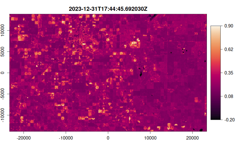
Step 5: Visualize as an Animated GIF

Create a function to plot each NDVI image, then render as an animated GIF:

# Create plotting function
ndvi_plot <- function() {
  # Start from image 10 stabilise median filter effect
  purrr::walk(10:tex_ndvi$n_items, function(i) {
    plot(
      tex_ndvi,
      item = i,
      col = hcl.colors(100, "Rocket"),
      title = "dttm", # Use datetime as title
      minmax_def = c(-0.2, 0.9), # Set NDVI color scale range
    )
  })
}

fs::dir_create("figure") # Create output directory if it doesn't exist

# Generate the animated GIF
gif_file <- gifski::save_gif(
  ndvi_plot(),
  gif_file = fs::path("figure", "ndvi_timeseries.gif"),
  width = 800, # Image width in pixels
  height = 450, # Image height in pixels
  delay = 0.1 # Delay between frames (seconds)
)